Thanks to Prof. Ian Horswill for the initial version of this assignment.
Advance Tutorial 1 Starter Files
Background
So far in class, we’ve mentioned two different ways of representing images in computers. The 2D graphics language discussed in Lecture 2 represents pictures in terms of primitive shapes and transformations applied to them. These kinds of graphics systems are called vector or object-oriented graphics. Examples of commercial vector graphics systems are so-called “draw programs” like Adobe Illustrator and Corel Draw, but also presentation graphics systems like PowerPoint and Keynote, and animation systems like Macromedia Flash (RIP).
Bitmap or raster graphics are the other major type of representation. They represent images as mosaics of colored squares called pixels (short for picture elements). Since nearly all video displays and printers ultimately form pictures using pixels, even vector graphics are generally rasterized (i.e. converted to a pixel-form) when displayed on the screen.
In this assignment, we’ll use a third kind of image representation: functions, aka procedures. Procedural images are a niche representation used primarily to represent the appearance of different kinds of materials like wood and marble in 3D computer graphics. In that context, they’re usually referred to as procedural textures, procedural shaders, or just shaders. Companies like Pixar have people who are wizards at writing shaders for different kinds of materials.
Intro
Start by opening the file adv_tutorial_1.rkt.
Now run the code in Tutorial 1 by pressing the Run button or typing Command-R. This will define a set of procedures that will let you write procedural shaders.
Note: If you’re on a recent-ish computer running macOS, your computer will ask if DrRacket can have permission to access the folder in which your
adv_tutorial_1.rktfile is stored. If you DENY that access, DrRacket won’t be able to load the two libraries we’ve provided for you:shading.rktandnoise.rkt.
Procedural shaders
Here’s the idea behind procedural shading. Ultimately, an image is just a variation of color over some surface where for any given position on the surface, there’s some specified color. In other words, a picture is in some sense a function from position to color. Rasters represent the function by breaking the surface up into little squares and assigning a color per square, but there’s nothing to prevent you from representing the image as a procedure that takes a location in the image as input and returns a color as output.
Recall that in Racket, you create functions using lambda expressions, expressions of the form:
(λ (argumentNames ...) returnValue)
The result of executing this expression is that it creates a function that takes its inputs and stashes them in variables with the specified argumentNames, and then runs the returnValue expression to compute the return value. If you like, you can then use define to give that function a name, but naming a function isn’t necessary, and in this exercise, you mostly won’t need to do it.
So given that a shader is a function that maps position to color or brightness, our basic syntax for it will be something like:
(λ (position)
  somethingToComputeTheColorForPoint)
where somethingToComputeTheColorForPoint can be any bit of Racket code you might want to write to compute the color for point.
Let’s limit ourselves to black and white images for the moment. That means the procedure only needs to specify a brightness for the point, rather than a full color. The procedure can represent the brightness as a number between 0 (black) and 255 (the brightest value the monitor can produce).
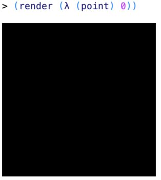
So a shader is a function that takes a position as an input and returns a number. The simplest example a shader is an image that’s black everywhere:
(λ (point) 0)
That is, no matter what the position is, the brightness is always zero. We’ve included a procedure with this assignment called render that that rasterizes a shader for you and displays it. So if we type:
(render (λ (point) 0))
Admittedly, that’s is not a terribly interesting image, so let’s try a one that starts black on the left and gets gradually brighter as it moves to the right. The code for this is just (λ (point) (point-x point)). point-x is a procedure that takes a point as input and returns its X coordinate. The X coordinates start at 0 on the left and increase as you move right.
Again, we can see the image by using render:
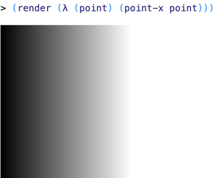
As it happens, render makes 300x300 images, so on the right hand side, the X the image stops getting brighter once the X coordinates get to 255 (because 255 is the maximum possible brightness). This is sometimes referred to as saturation – the brightness goes outside the range that the display device can generate. The system does the same thing with “negative” brightnesses – it just treats them as 0.
So we can get what draw programs sometimes call a “gradient” when we use the X coordinate for brightness. We can get what they call a “radial gradient” by taking the magnitude of the point (its distance from (0,0), the upper-left-hand corner of the image):
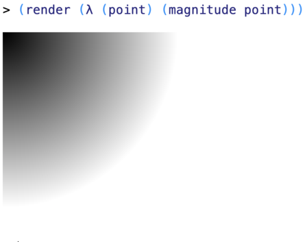
Here we use the magnitude procedure to get the magnitude of the point (distance from the upper-left corner), and again, the brightness saturates once we get more than 255 pixels from (0,0), that corner.
Arithmetic with points
Points can be used in arithmetic operations. The
point-*procedure multiplies both coordinates of the point by the number. So multiplying the point (1,2) by 2 gives you the point (2,4). Multiplying points by numbers has the effect of stretching them away from the origin (the upper-left corner), but keeping their direction relative to the origin the same.The
point-+procedure adds the coordinates of two points together, so that(1, 2)+(5, 3)=(6, 5).You can also subtract points using the
point--procedure.
Alternatively, we could get a kind of concentric ring structure, like wood grain, if we took the sine of the distance rather than the distance itself as the brightness:
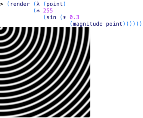
Here we multiply the distance by a fudge factor (0.3) that we can use to adjust the spacing of the rings (bigger numbers mean more rings closer together), and we multiply the output of sin by a fudge factor to change the brightness of the image (bigger numbers mean brighter).
Noise functions
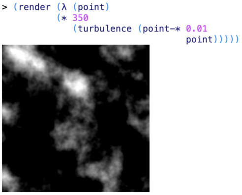
Procedural shading starts to get more interesting when we use noise functions. Noise functions are functions that vary “randomly” in some controlled way. The most popular noise function is based on the Perlin noise function, and is called the turbulence function. It’s used to create clouds and marble textures. Here’s an example of Perlin noise:
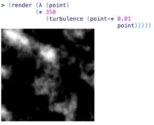
Again, we multiply point by a fudge factor (0.01) to adjust the scale of the image. We multiply the output of the turbulence function by a different number (in this case 350) to adjust the brightness of the image (turbulence produces small numbers, which correspond to dark pixels). We can make the texture finer by increasing the multiplier on point from 0.01 to 0.02:
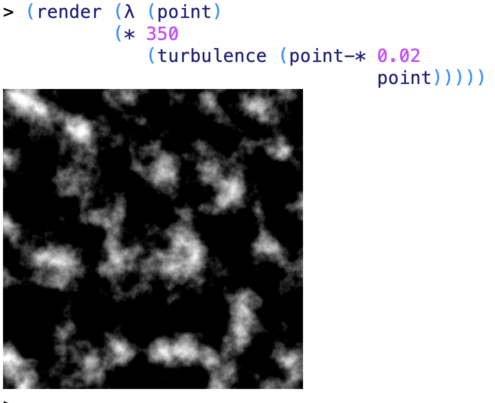
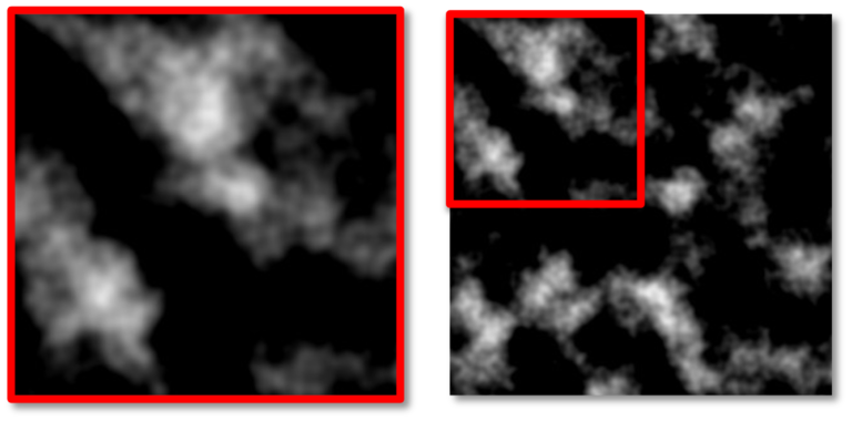
Now everything from the previous image is shrunken into the upper left hand corner of the new image:
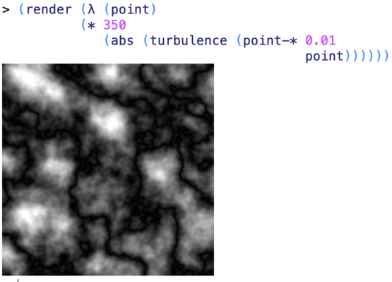
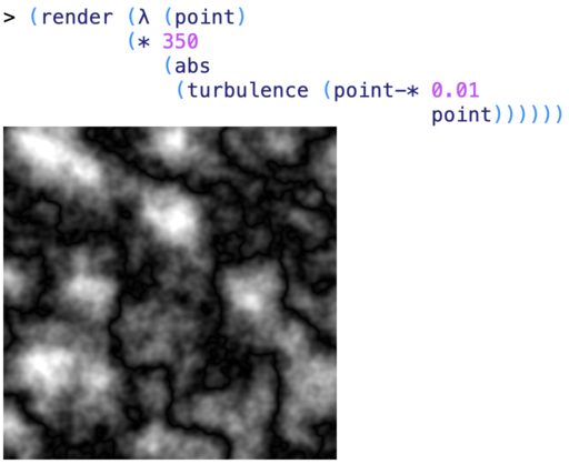
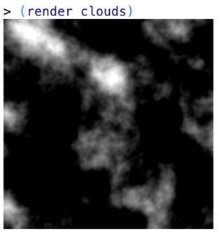
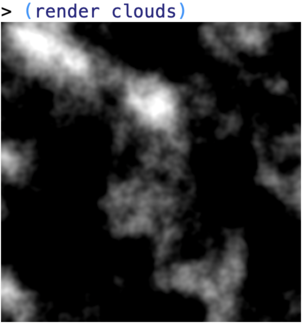
The turbulence function is often used to render clouds. A standard turbulence function produces numbers for its output between -1 and +1 (actually, between about -0.8 and +0.8). Since the render procedure treats the negative “brightnesses” as just meaning normal black (the same as 0), the big black regions between the clouds are the regions where the turbulence function is returning zero or negative numbers. But we can make them visible, by rendering the absolute value of the turbulence function, so the negative regions become positive. This gives us something closer to a marble texture, and indeed, this is how marble surfaces are often rendered in computer graphics:
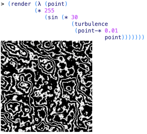
Alternatively, we can use a sin function instead of abs to get something that looks almost like a topographic map:
Normal version
Absolute value - fills in clouds between clouds (sort of like marble)
Sine - clouds become contour maps
Part 1. Writing your own shaders
For this part, we just want you to experiment with writing shaders and see what kinds of images they generate. There’s no fixed goal for this. Just try playing around.
Part 2. Writing procedures that modify shaders
Now that you’ve had a chance to experiment with writing shaders, we’re going to write procedures that work with shaders. These are procedures that take shaders as inputs and produce new shaders as outputs.
- Write a procedure,
brighten, that takes as inputs a shader and a multiplier (a number), and returns as output a new shader whose output at any given point is the simply the output of the original shader at that point times the multiplier. So if we brighten a shader by 2, we get a new shader whose output is the original shader’s output times 2 (i.e. twice as bright).
This kind of thing can be hard to communicate in text. So here’s a concrete example. We’ve included the cloud shader above under the name clouds. If you run (brighten clouds 2), you should get the the same clouds, only twice as bright. If you run (brighten clouds 0.5), it should be half as bright:
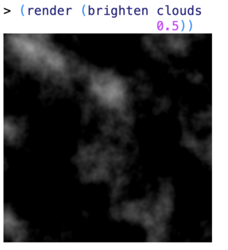
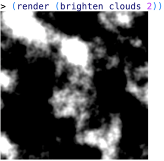
So where clouds returns 50 for some point (i.e. 50 units of brightness), (brighten clouds 2) should return 100 and (brighten clouds 0.5) should return 25.
To do this problem, you want to write brighten so that it returns a shader. But a shader is just a procedure that takes a point as input and returns a brightness. So you want to write a procedure whose output is itself a procedure, in particular a λ expression:
(define brighten
   (λ (shader multiplier)
     (λ (point)
       something)))
The (λ (point) something) here is the new shader being returned by brighten. It takes an argument, point, as input and then needs to compute the brightness for the image at that location. How does it compute that brightness? We’ll it’s just the brightness of the original shader times multiplier. But how does it know what the brightness of the original shader is? It just calls it: (shader point).
- Now write a procedure,
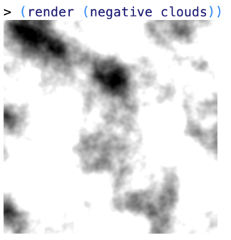
negative, that gives you a negative image (in the sense of a negative from old film camera) of a shader, so that what was white in the original shader is now black, and what was black is now white: if the original shader returns 0 at a point, the new one should return 255 and vice versa. More generally, if the original shader returns some numberxat a point, the new shader should return the number255-x. Again, here’s an example with clouds:
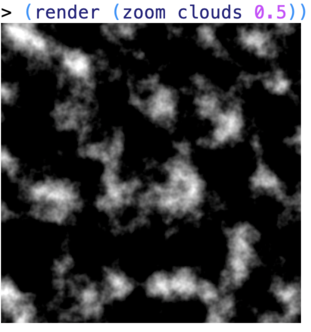
- Now write a procedure,
zoom, that takes a shader and a scale factor as input, and it returns a shader that’s magnified (in the sense of grown, not brightened) by that factor, like this:
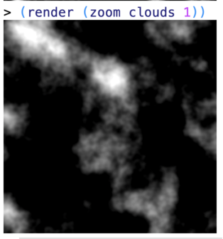
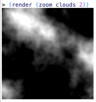
zoom is like brighten, except that instead of multiplying the output of the original shader (that is, multiplying the brightness), it divides its input. So in order words, instead of calling shader with point as its input, it calls it with:
(point-/ point scale-factor)
as its input. point-/ is a procedure that makes a new point from the original one, but divides each coordinate by the scale factor.
You might think that you’d want to multiply the point by the scale factor rather than divide by it (I did when I first wrote it). But try both (or think it through) and you’ll see that you actually want to divide.
- Now write a procedure,
slide, that shifts a shader’s image by a specified amount. In particular, slide should take a shader and a point as inputs, and return a new shader that looks like the original, but where whatever was previously at (0,0) is now shifted to the specified point. For example:
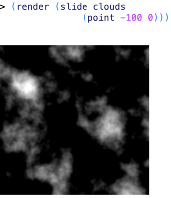
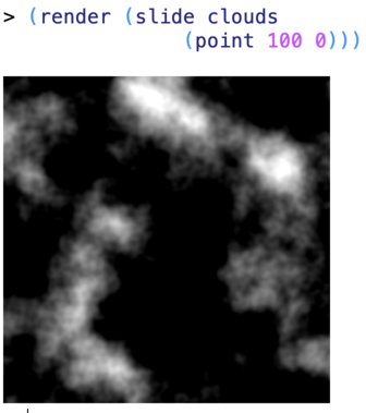
You solve this one like zoom, in that you make a new shader that calls the old shader with a different point as input. However, in this case, instead of calling it with (point-/ point scale-factor) as its input, you call it with (point-- point offset), where offset is the amount we want to shift the image by. Again, you might think you’d want to add the offset to the original point, but if you try it you’ll see that subtracting is the right thing to do.
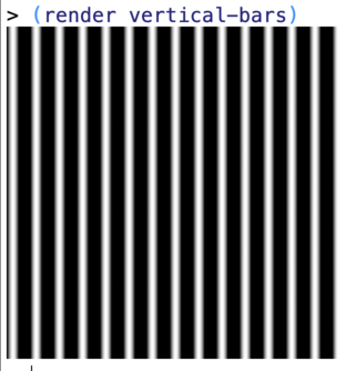
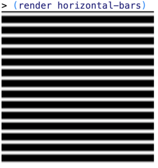
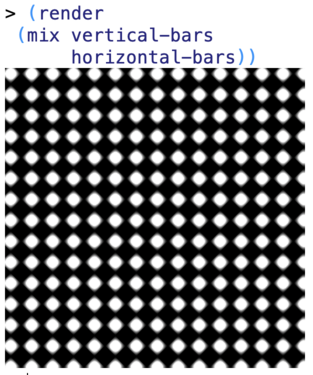
- Finally, write a procedure,
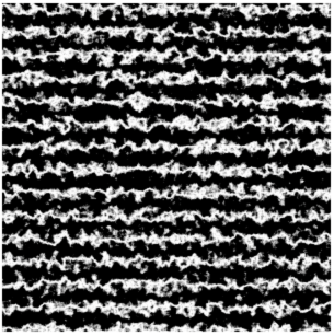
mix, that takes two shaders as inputs and returns a new shader whose brightness at a point is the average of the brightnesses of the two shaders, so that it does a kind of double-exposure. Here we’ll demonstrate it with two other shaders we’ve included with the assignment file,vertical-barsandhorizontal-bars, that just create sine wave patterns:
Part 3. Freestyle
Now just play around and have fun. See what kinds of images you can make!
Part 4. Extra Advanced
Write a procedure, morph, that takes a shader and a function as input and returns a new shader based on the original shader, but deformed based on the function. Here’s what we mean. If you say (morph shader f), where f is function from points to points, then you should get back a new shader who’s value at a point p is just (shader (f p)).
Morphing is used a lot in graphics. For example, zooming and shifting are just special cases of morphing:
(define zoom
   (λ (shader magnification)
      (morph shader
             (λ (p) (point-* magnification p)))))

(define shift
   (λ (shader point)
      (morph shader
             (λ (p) (point-- p point)))))
But we can also do some more sophisticated operations. For example, the noise-vector procedure makes a random vector that can be added to a point, shifting it slightly around. If we use this to morph an image, we get a crinkling effect:
(define crinkle
     (λ (shader)
       (morph shader
              (λ (p)
                (point-+ p
                         (noise-vector p 10 0.1))))))

(render (crinkle horizontal-bars))
In the code above, 10 is a multiplier that controls how big the noise vector is. Make it bigger and the image will get more distorted. Make it smaller, and it will become less distorted. The 0.1 is a scale factor that controls how fast the noise vector changes from pixel to pixel. The bigger it is, the faster it changes, and so in a certain sense the smaller the “scale” of the distortion. I know that’s confusing to read in English, but if you play with the numbers, you’ll get the idea.
Shaders
Much of the appearance of objects in 3D graphics comes from “texture mapping” where texture images are “wrapped” around objects like wallpaper. The exact process for this is outside the scope of this class, but the basic idea is the artist designing an object chooses a texture image for each object, and assigns a location in the image to each point on the object’s surface. When the system renders (draws) the object, it determines where on the screen the object is, and for each screen pixel in that region, it determines the coordinates of that pixel on the surface of the object, then from that determines the coordinates in the texture image. The system then runs the shader to determine the color that should appear at that point.
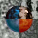
The image above (originally from Ken Perlin’s web site that’s no longer online) shows four different noise textures, both as flat images, and as textures mapped onto the surface of a sphere.
Submitting
Regardless of how you choose to complete the assignment, you MUST submit the file you worked on to Canvas. Do that now. Since you're working on an advanced tutorial, make sure the string adv appears somewhere in your file name.
Please refer to the original Canvas assignment for exact details on how to prove your attendance.